Special Ordered Sets
Special Ordered Sets (SOSs) are ordered sets of variables, where only one/two contiguous variables in this set can assume non-zero values. Introduced in [BeTo70], they provide powerful means of modeling nonconvex functions [BeFo76] and can improve the performance of the branch-and-bound algorithm.
- Type 1 SOS (S1):
In this case, only one variable of the set can assume a non zero value. This variable may indicate, for example the site where a plant should be build. As the value of this non-zero variable would not have to be necessarily its upper bound, its value may also indicate the size of the plant.
- Type 2 SOS (S2):
In this case, up to two consecutive variables in the set may assume non-zero values. S2 are specially useful to model piecewise linear approximations of non-linear functions.
Given nonlinear function \(f(x)\), a linear approximation can be computed for a set of \(k\) points \(x_1, x_2, \ldots, x_k\), using continuous variables \(w_1, w_2, \ldots, w_k\), with the following constraints:
Thus, the result of \(f(x)\) can be approximate in \(z\):
Provided that at most two of the \(w_i\) variables are allowed to be non-zero and they are adjacent, which can be ensured by adding the pairs (variables, weight) \(\{(w_i, x_i) \forall i \in \{1,\ldots, k\}\}\) to the model as a S2 set, using function add_sos(). The approximation is exact at the selected points and is adequately approximated by linear interpolation between them.
As an example, consider that the production cost of some product that due to some economy of scale phenomenon, is \(f(x) = 1520 * \log x\). The graph bellow depicts the growing of \(f(x)\) for \(x \in [0, 150]\). Triangles indicate selected discretization points for \(x\). Observe that, in this case, the approximation (straight lines connecting the triangles) remains pretty close to the real curve using only 5 discretization points. Additional discretization points can be included, not necessarily evenly distributed, for an improved precision.
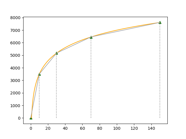
In this example, the approximation of \(z = 1520 \log x\) for points \(x = (0, 10, 30, 70, 150)\), which correspond to \(z=(0, 3499.929, 5169.82, 6457.713, 7616.166)\) could be computed with the following constraints over \(x, z\) and \(w_1, \ldots, w_5\) :
provided that \(\{(w_1, 0), (w_2, 10), (w_3, 30), (w_4, 70), (w_5, 150)\}\) is included as S2.
For a complete example showing the use of Type 1 and Type 2 SOS see this example.